I built a digital chemical world you can disturb

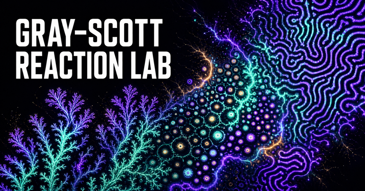
The first thing that got me was how alive it looked. A small chemical seed expanded, pinched in the middle, split, and crowded itself into a field of glowing cells. Nothing in the code said, “draw a cell here.” The code only described how two concentrations should react and spread. The shapes arrived on their own.

I have always liked trippy visuals, strange interactive systems, generative art, and that point where science stops being something you observe from a distance and becomes something you can actually play with. I wanted to understand reaction-diffusion systems well enough to feel their behavior, not just read about it, so I built the Gray-Scott Reaction Lab.

It is a full-screen browser experiment where you disturb a simulated chemical field and watch it reorganize. The controls let you change the chemistry while it is running, move between known pattern regimes, alter the way the chemicals diffuse, and save whatever appears. It now lives in my Projects alongside the businesses and systems I have built, but it is intentionally more playful than most of my work.

Why I made it

Most of my day-to-day systems are designed to make something predictable: a workflow should run, a team should know what happens next, a content system should produce consistent output. Reaction-diffusion is almost the opposite kind of pleasure. The rules are precise, but the result is surprising.

I wanted an experiment where the interface did not simply display a scientific model. It had to invite interference. You should be able to touch the field, introduce a disturbance, and then step back while the system interprets what you did. Sometimes your mark becomes a colony. Sometimes it breaks into moving fragments. Sometimes the surrounding chemistry consumes it completely.

That feedback makes the model understandable in a way a static diagram cannot. The interaction is not “drawing” in the usual sense. It is closer to changing the local conditions in a tiny artificial world and seeing whether the world accepts the change.

Two chemicals and one surprisingly expressive loop

The Gray-Scott model tracks two chemical concentrations, usually called U and V. U is fed into the system. V consumes U in a reaction that produces more V. At the same time, V is removed, and both chemicals diffuse across the surface at different rates.

In compact form, the model is:

U diffuses, is consumed by the reaction UV², and is replenished by feed rate F. V diffuses, grows through the same reaction, and is removed according to F + k.

That is the whole engine. There is no hidden library of coral shapes or spot animations. Each point in the lattice repeatedly looks at its neighbors, calculates diffusion, applies the reaction, feed, and removal terms, then advances by one small timestep. Run that calculation across hundreds of thousands of cells, thousands of times, and structure begins to appear.

The model is an established piece of reaction-diffusion research. John E. Pearson's 1993 paper, Complex Patterns in a Simple System, mapped many of its now-famous behaviors. Robert P. Munafo later studied localized moving structures in a narrow part of the parameter space. I did not invent those equations or their scientific classifications. What I built is the interactive browser implementation: the rendering pipeline, controls, preset curation, disturbance behavior, visual palettes, accessibility, and local export tools.

The smallest numbers make the biggest changes

Two controls do much of the visible work. F controls how quickly U is replenished. k controls how quickly V is removed. Their useful values sit in a narrow numerical range, and changing either by a few thousandths can transform the entire culture.

One region produces stable spots. Another grows long stripes that bend away from one another. Elsewhere, cells repeatedly divide, wave fragments collide, or small localized patterns move across the field. The behavior is not encoded in the preset name. A preset only loads a set of parameters, boundary conditions, a starting concentration, and a visual palette. The model still has to grow the result.

I gave the presets readable labels such as Coral, Worms, Bubbles, Mitosis, Moving Spots, Maze, and Waves, while keeping established Greek labels and references where they matter. The descriptions explain what to look for without pretending every run will produce an identical picture. This is a dynamic system, not a video filter.

Making a disturbance instead of drawing a line

The interaction took more thought than I expected. An early version treated pointer movement too much like a conventional paintbrush. It left a continuous trail, which made very different chemical regimes feel similar at first. Worse, a mostly empty initial field asked visitors to understand the model before it gave them anything interesting to watch.

The current brush injects a controlled series of soft, slightly irregular concentration splats. Fast movements are interpolated so they do not leave large gaps, but the spacing is limited so one quick swipe does not flood the lattice. Brush material, radius, and strength still matter. Pen pressure can add a small amount of nuance when the browser provides it, but mouse, trackpad, touch, and stylus all work without requiring pressure data.

Most importantly, the marks change U and V. They are not cosmetic pixels placed on top of the image. Once the disturbance enters the simulation, the selected parameters decide its future. That distinction is the entire experience.

Inside the browser laboratory

The main simulation runs in WebGL 2. Two floating-point textures hold the current concentrations, and the browser alternates between them while applying the Gray-Scott update in a fragment shader. This “ping-pong” approach lets the GPU advance every lattice cell in parallel without reading the field back to JavaScript.

There is also a typed-array Canvas fallback for browsers that cannot render to the required floating-point textures. Larger lattice options automatically receive tighter speed limits, and the animation loop caps catch-up work so a slow device cannot trap itself trying to calculate an ever-growing backlog. Reduced-motion preferences start the experiment paused with glow disabled.

The numerical method is deliberately clear rather than exotic: explicit Euler integration and a common weighted nine-point lattice Laplacian. The default diffusion multipliers preserve a 2:1 U-to-V ratio. The lab also includes a classical case from the paper supplied with the project, while noting that paper's fractional-diffusion extension rather than quietly claiming to implement it.

Growing and keeping a world

You can start with a preset, drag through the field, and leave it alone. Or you can pause, place a seed precisely, advance one timestep at a time, switch the displayed signal, change palettes, toggle glow, and adjust diffusion or boundary behavior. Reset returns to a seed designed for the active culture. Randomize creates a fresh set of islands. Clear removes the disturbance entirely and reveals an important fact: the perfectly uniform state has nothing to react to.

PNG exports can stay clean or carry a small specimen label with the actual simulation step, preset, feed rate, kill rate, lattice size, and date. I like the label because it treats the output as the record of a computational specimen rather than a generic wallpaper. Short recordings remain clean field captures, and everything is generated locally. Nothing is uploaded.

What building it taught me

First, initial conditions are part of the design. Two simulations with identical F and k values can behave differently because of how and where the chemistry was disturbed. A good preset therefore needs more than the right numbers. It needs a starting culture that gives that regime a reasonable chance to reveal itself.

Second, scientific accuracy and playful design are not opposites. The model became more fun when the interaction reflected the chemistry more honestly. Replacing a generic trail with concentration splats improved both the feel and the explanation.

Third, emergence is a useful systems lesson outside this simulator. The final shape is not controlled directly. It comes from rules, feedback, local interactions, constraints, and time. That is also why I keep returning to systems in my business work. In Buying Tools Before Systems Cost Me Three Times, the subject is much less psychedelic, but the underlying idea is related: outputs are downstream of the system that produces them.

Computational Studio 01

I am calling this Computational Studio 01 because I want room for more experiments like it: small, interactive studies where code becomes a material and visitors can learn by changing the system. Cellular automata, strange attractors, particle ecosystems, evolutionary simulations, artificial life, and generative architecture all belong somewhere on that list.

I am not building a grand index before the work exists. For now, this is simply the first specimen. It is a place to grow a world from two virtual chemicals, disturb it, watch what survives, and save the result when something strange appears.

Open the Gray-Scott Reaction Lab

Research Confidence

This article is based on:

• The classical Gray-Scott equations and parameter map published by John E. Pearson in 1993
• Robert P. Munafo's published study of localized moving Gray-Scott patterns
• The supplied 2026 paper's classical numerical case and its documented fractional extension
• Direct implementation and numerical observation in the browser simulator; future Computational Studio topics remain proposals

Confidence Level: Experimental

Frequently asked questions